Log-normal model for solvency 2 USP
Introduction
Under Solvency 2 framework, insurance compagnies can calculate undertaking specific parameters to modify their application of the standard formula, as dictates Commission-Européenne (2014) . One of thoose calculations methods uses a log-normal model that’s quite interessante to analyse. We will here analyse this model in a mathematical sense, and then use it on simulated data (i’m not an insurence compagny !) for a quick exemple of application.
The log-normal model
Under the standard formula, agregation of risk depend on variation coefficients \(\sigma\)’s that are use to asses the variability of next year risks. In our case, this parameter can be understood as the ratio between the standard variation of next-year boni-mali’s divided by this year Best estimate. The calculation by an insurance compagny of an USP for reserve risk is ruled by one of 2 models, we will here focus on the first one.
This model supposes (on top of a log-normal hypohtesis) a linear relation between 2 factors :
- The Best estimate at end of the year, denoted here \(x_t\) for year \(t\)
- The same Best estimate plus paiements done during the year, denoted here \(y_t\)
and this relation should hold \(\forall t \in \{1,..,T\}\). We will also denote :
- \(\sigma\), the variation coefficient of the risk, which is the parameter we want to assess.
- \(\delta \in [0,1]\), mixing parameter
- \(\beta\), the expected ,
- \(\gamma = ln(\frac{\sigma}{\beta})\).
The log-normal model proposed by Solvency 2 states under thoose notations that :
- \((H1)\) : \(\mathbb{E}(y_t) = \beta x_t\), i.e losses are proportional to premiums through a coefficient \(\beta\).
- \((H2)\) : \(\mathbb{V}(y_t) = \sigma^2\left((1-\delta)\bar{x}x_t + \delta x_t^2\right)\), where \(\bar{x} = \sum_{t=1}^{T} x_t\)
- \((H3)\) : \(y_t \sim log\mathcal{N}(\mu_t,\omega_t^2)\), \(y_t\) follows a log-normal.
Under \((H123)\), we are looking for a maximum likelyhood estimate of \(\sigma\). The likelyhood of the model is here given by :
\[\mathcal{L}^1(y_1,...,y_T,\beta,\sigma) = \prod\limits_{t=1}^{T} \frac{1}{y_t \omega_t \sqrt{2\pi}} exp\left\{\frac{-(ln(y_t)-\mu_t)^2}{2\omega_t}\right\}\]
Maximising the log of this likelyhood, we can found an estimate for the \(\sigma\) paramter. Note that this parameter can be extracted from the log-likelyhood. Indeed, if we write :
\[\pi_t\left(\hat{\delta},\hat{\gamma}\right) = \frac{1}{ln\left(1+e^{2\hat{\gamma}}\left((1+\hat{\delta})*\frac{\bar{x}}{x_t}+\hat{\delta}\right)\right)}\]
and if we estimate \(\hat{\delta},\hat{\gamma}\) by maximising the log-likelyhood, Roos (2015) prooved that this was equivalent to minimise the function proposed by Solvency II in Commission-Européenne (2014) , given by :
\[\sum\limits_{t=1}^{T} \pi_t\left(\hat{\delta},\hat{\gamma}\right)\left(ln\left(\frac{y_t}{x_t}\right) + \frac{1}{2\pi_t\left(\hat{\delta},\hat{\gamma}\right) } - \frac{\frac{T}{2} + \sum\limits_{t=1}^{T} \pi_t\left(\hat{\delta},\hat{\gamma}\right) ln(\frac{y_t}{x_t})}{\sum\limits_{t=1}^{T} \pi_t\left(\hat{\delta},\hat{\gamma}\right)}\right)^2 - \sum\limits_{t=1}^{T} ln\left(\pi_t\left(\hat{\delta},\hat{\gamma}\right)\right)\text{,}\]
We then found our maximum likelyhood estimate for \(\sigma\) in \(\hat{\sigma}\left(\hat{\delta},\hat{\gamma}\right)\), defined as :
\[\hat{\sigma}\left(\hat{\delta},\hat{\gamma}\right) = exp\left\{\hat{\gamma} + \frac{\frac{T}{2} + \sum\limits_{t=1}^{T} \pi_t\left(\hat{\delta},\hat{\gamma}\right) ln(\frac{y_t}{x_t})}{\sum\limits_{t=1}^{T} \pi_t\left(\hat{\delta},\hat{\gamma}\right)}\right\}\text{.}\]
For th sake of simplicity, we’ll take here data that are old enough (15points) to have the needed credibility so that this estimator is our USP. We refere to Rouchati (2016),Gauville (2017) and to the standard formula for more details about this.
A funny fact : Finaly, the delegated regulation give us a “unbiaising” formula :
\[\hat{\sigma} = \hat{\sigma}\left(\hat{\delta},\hat{\gamma}\right) \sqrt{\frac{T+1}{T-1}}\]
But as remarked Roos (2015) (see appendix A), this unbiaising factor is not optimal under model hypothesis ! Furthermore, a right factor can be calulated.
If you want more details about the theory underlying this model, e.g proof f the estimators, see BEAUNE (2016) or Roos (2015).
Generating dummy dataset.
We will here work on a simultaed dataset of best estimates \(x_t\) and \(y_t\) on a a window of 15years. Let’s generate them not too far away from the model :
df <-
  data.frame(year = 1:15) %>%
  mutate(
    x = seq(10000,20000,length=15)+rnorm(15,0,500),
    y = 1.05*x + exp(rnorm(15,0,1))
)| year | x | y |
|---|---|---|
| 1 | 10103.66 | 10609.56 |
| 2 | 10383.26 | 10905.38 |
| 3 | 11057.49 | 11610.60 |
| 4 | 12602.01 | 13232.34 |
| 5 | 12797.13 | 13440.30 |
| 6 | 14051.94 | 14758.50 |
| 7 | 13961.17 | 14660.51 |
| 8 | 14868.41 | 15613.67 |
| 9 | 16171.93 | 16981.48 |
| 10 | 16634.91 | 17469.45 |
| 11 | 16335.36 | 17153.03 |
| 12 | 17828.52 | 18720.15 |
| 13 | 18942.66 | 19890.51 |
| 14 | 18620.45 | 19552.54 |
| 15 | 19416.84 | 20388.04 |
Checking model hypohtesis.
The model has fundamentaly 2 hypothesis :
- Log-normality of \(y_t\) serie,
- Linearity between \(y_t\) and \(x_t\)
Log-normality of \(y_t\)
To study the first one, we propose to use a Shapiro-wilk test, given by Shapiro and Wilk (1965), which gives a test statistic and a p-value as follows :
| Statistic | p-value | |
|---|---|---|
| \(x_t\) | 0,9355064 | 0,3292087 |
| \(y_t\) | 0,9355259 | 0,3294248 |
We also propose to do a Kolmogorof-smirnoof test. note that it’s equivalent to test normality of the log or log-normality directly. This gave the following results :
| Statistic | p-value | |
|---|---|---|
| \(x_t\) | 0,1475037 | 0,8541257 |
| \(y_t\) | 0,1474602 | 0,8543577 |
Thoose 2 test confirm the log-normal hypohtesis. Well we simultaed data for it, so it’s kinda easy to pass the tests. But on real data, those test are powerfull. We finaly propose a qqplot for \(y_t\). For log-normal law, we usualy pass the qqplot at log-scale to see regularly espaced points and a more readable plot :

The alignement is not perfect, but there is’nt so much data. Thoose tests confirm the log-normality for \(y_t\), but also for \(x_t\) which is not asked by the model. I did it to see how much it is easy to pass test when there are only 15 points.
We therefore accept the log-normality for \(y_t\)
Linearity between \(y_t\) and \(x_t\)
The linearity hypthesis on \(y_t\) can be translated into normality of residuals given by :
\[r_t = \frac{ln(y_t) - \hat{\mu}_t}{\hat{\sigma}_t}\text{,}\]
where \(\mu_t\) and \(\sigma_t\) are the parameters of the underlying log-normal. Note that we have by definition of a log-normal that \(\mathbb{E}(y_t) = e^{\mu_t + \nicefrac{\sigma_t^2}{2}}\) and \(Var(y_t) = (e^{\sigma_t^2}-1)e^{2\mu_t+\sigma_t^2}\), see wikipedia for a proof.
Residuals obtained here are therefore supposed to follow a gaussian white noise, i.e a gaussian process without autocorrelations. If norallity of residuals is already OK (equivalent to log-noramlity of \(y_t\)), tests corresponding to the white noise (not gaussian) are done following the auto_arima function in R :
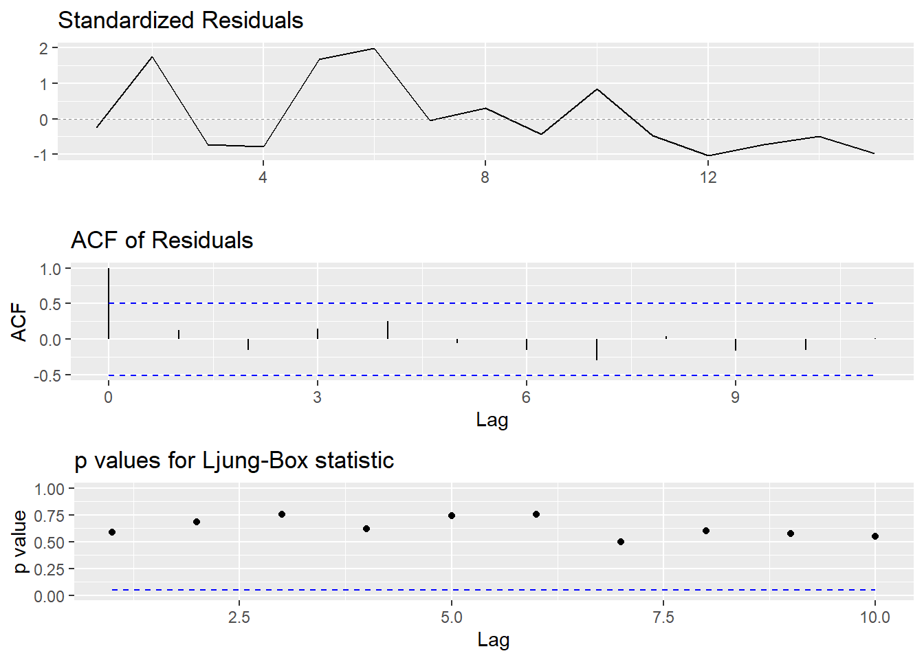
We see that residuals satisfy a white-noise hypothesis. Therefore, residuals can reasonably be though as comming out of a gaussian white noise process.
Finaly, we propose to calculation confidence interval for predicted values of \(y_t\) under model hypothesis (log-normality and esperance/variance stimated by the model). The regression line is as follows, at a confidence \(\alpha = 0.05\).
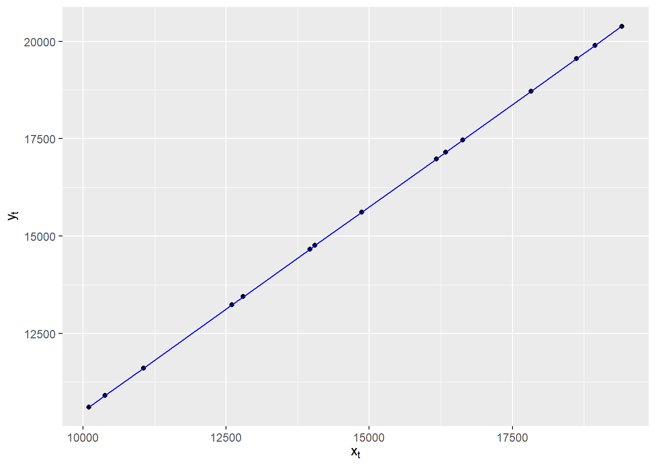
The facts that data are inside the confidence interval puhs us forward into validation of hypothesis.
Results from the model
Since the hypohtesis have been checked, let’s now calculate the \(\sigma\) parameter under theese hypothesis. The application of maximum likelyhood estimation is done through the optim function in R, via the Newton-Raphson algorythme. The algorythme converge realy fast because we dont have much data. Here is the result :
| \(\hat{\gamma}\) | \(\hat{\delta}\) | \(\hat{\sigma}(\hat{\delta},\hat{\gamma})\) | \(\hat{\sigma}\) | |
|---|---|---|---|---|
| Estimations | -9,36221 | 0 | 0.00902% | 0.00964% |
Note that \(\hat{\delta}\) is borned between \(0\) and \(1\).
Although we took stupid inputs and therefore results are awfull, this model is very satisfying beacause it’s high level, in the sense of programing level : it uses directly best estimates from the compagny and therefore takes into account everything that was taken into acount during calulation of thoose best-estimates, including the whole reserving process of the compagny.
It’s therefore a great method to juge the quality of reserving from a compagny. However, the method takes into account very few data points and is therefore unprecise..
Maybe some time we’ll talk about better method to assess reserving risk !
References
BEAUNE, Lucile. 2016. “Estimation des paramètres de volatilité propres aux assureurs non-vie.” Mémoire d’Actuariat.
Commission-Européenne. 2014. “Règlement Délégué (UE) 2015/25 de La Commission U 10/10/2014.”
Gauville, Rémi. 2017. “Projection Du Ratio de Solvabilité : Des Méthodes de Machine Learning Pour Contourner Les Contraites Opérationnelles de La Méthode Des SdS.” Mémoire d’Actuariat.
Roos, Mordehai. 2015. “Utilisation des Undertaking Specific Parameters avec une base de données santé,” November, 106.
Rouchati, Faries. 2016. “Projection Du Ratio de Solvabilité d’un Assureur Retraite : Les Méthodes Paramétriques (Curve Fitting et Least Square Monte Carlo) Peuvent-Elles Se Substituer à La Méthode Des Similations Dans Les Simulations ?” Mémoire d’Actuariat.
Shapiro, S S, and M B Wilk. 1965. “An Analysis of Variance Test for Normality (Complete Samples),” 22.
Oskar Laverny
Maître de Conférence
What would be the dependence structure between quality of code and quantity of coffee ?